
This page is not intended to provide complete information for data analysis. We can not expect a unique model or method to fit well for all type of data. This is a collection of commands or a rough collection of commands to use some R packages to fit a specific model or to analyse a certain type of data. This page is intended to remind myself for some commands rather than searching in R help pages. I hope this page (Items Covered) will grow with time to make my life lot easier!
1. Create and Edit Maps
To create a map, one needs to get the shape file. Here is an R script that will allow you to create a map.
library(foreign)
library(maptools)
library(PBSmapping)
myShapeFile<- importShapefile("C:/Users/username/CED07aAUST_region.shp", readDBF=TRUE)
str(myShapeFile)
plotPolys(myShapeFile, xlab="Longitude", ylab="Latitude")
plotPolys(myShapeFile, col=gray(c(1:n.ced)/n.ced), xlab="Longitude", ylab="Latitude")
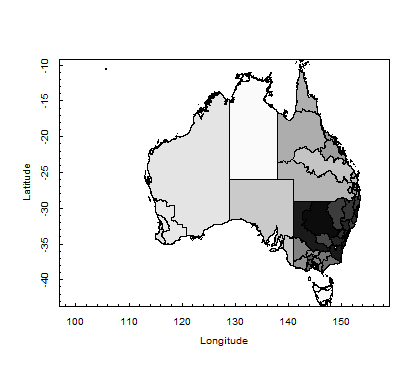
Figure: Commonwealth Electoral Divisions (CED)
You may use many other options to edit this graph by placing symbols for certain locations, events in some places, co-ordinates, values, and texts. You can also use google map to call from R and edit the map accordingly based on your needs. I hope to update this section in near future!
2. Panel Data Analysis
Panel data format, let’s call the data file a data.frame in R. This a practical example but for theories you should consult any standard textbook.
How does a panel data.frame look like? Here is a typical panel data.frame.
firm  year  cost  profit harvest
1     1990   12.6  4.2   15.3
1     1991   12.9  4.0   16.2
:     :      :     :     :
1     2010   14.2  2.5   9.5
2     1990   6.6   1.8   8.6
2     1991   5.3   1.9   7.9
:     :      :     :     :
10    2010   20.1  7.5   30.2
Fit a fixed effect and random effect panel regression model, and check the feasibility of random effect model over the fixed effect model by using the Hausman test. Finally, check the presence of heteroskedasticity and update the standard errors by heteroskedasticity consistent (HC) estimates.
 firms <- readRDS("C:/Users/.../firms.rds") # call the data frame as an R data file
 library(plm)
 library(tseries)
 library(lmtest)
 adf.test(firms$profit, k=2) # if p-value<0.05, there is no unit root and is stationary
 # we want to fit the model: fit<- log(profit) ~ log(harvest) + log(cost)
 fit<-log(profit) ~ log(harvest) + log(cost)
 bptest(fit, data = firms, studentize=F) # p-value<0.05 then heteroskedasticity is present
 model1 <-plm(fit, data=firms, model="within", effect="time", random.method="amemiya")
                       # model1 is a fixed effect model
 model2<- plm(fit, data=jobs, model="random", effect="time", random.method="amemiya")
                       # model2 is a random effect model
 summary(model1)
 summary(model2)
 phtest(model1, model2) # if p-value<0.05, then use the fixed effect model
 coeftest(model2) # original coefficients but there is heteroskedasticity
 coeftest(model2, vcovHC) # update with heteroskedasticity consistent estimates
3. Count Response Data Analysis
Let us consider a data.frame in R where the data frame ModelData consists of several variables. Our objective here is to fit a count response model for number of hospital admission in response to extreme climatic factors (diurnal temperature change, relative humidity, at-risk warning based on climatic condition and air quality).
fitData = data.frame( station = factor(ModelData$StationCode),
                      time = ModelData$time,
                      adcount = ModelData$admcount,
                      dtempc = ModelData$diurnalTempChange,
                      arwarn = factor(ModelData$atriskWarning),
                      rhum = ModelData$relativeHumidity
                     )
library(MASS)
PoissonModel = glm(adcount ~ arwarn + dtempc + rhum, data=fitData,
                   family=poisson(link = "log"))
     # summary(PoissonModel)
glmpoisson.out = round(summary(PoissonModel)$coefficients,4)
     # construct a table of estimates
glmpoisson.est = cbind(Estimate = glmpoisson.out[,1],
                       expEstimate = exp(glmpoisson.out[,1]),
                       z = glmpoisson.out[,3] )
     # Sometimes a negative binomial model is used, especially when
     # there are frequent zero counts as can be in hospital admission
NBModel = glm.nb(adcount ~ arwarn + dtempc + rhum, data=fitData)
     # summary(NBModel)
glmNB.out = round(summary(NBModel)$coefficients,4)
     # construct a table of estimates
glmNB.est = cbind(Estimate = glmNB.out[,1],
                  expEstimate = exp(glmNB.out[,1]),
                  z = glmNB.out[,3] )
4. Count Response Panel Model (Panel Generalized Linear Model)
In Section 3, we have fitted count response models to predict the number of hospital admissions in response to climatic drivers. We also notice that there is another variable StationCode in the data set. Thus the data set can be thought as a panel data frame and a linear panel fitted in Section 2 is not suitable for this data set. We need to fit a count response panel data model (panel generalized linear model) to this data.
library(pglm)
     # construct panel data frame
pglmData = pdata.frame( fitData, index = "station", drop.index = FALSE)
     # type of models to choose: "within", "random" and "pooling"
     # two options for family to choose from: "poisson" and "negbin"
pglmModel1 = pglm( adcount ~ arwarn + dtempc + rhum, fitData,
               family = poisson, model = "within", method = "nr")
     # summary(pglmModel1)
pglmModel2 = pglm( adcount ~ arwarn + dtempc + rhum, fitData,
                 family = poisson, model = "random", method = "nr")
     # summary(pglmModel2)
pglmModel3 = pglm( adcount ~ arwarn + dtempc + rhum, fitData,
                 family = poisson, model = "pooling", method = "nr")
     # anova(pglmModel1, pglmModel2)
pglmModel4 = pglm( adcount ~ arwarn + dtempc + rhum, fitData,
                 family = negbin, model = "within", method = "nr")
     # summary(pglmModel4)
5. Machine Learning Methods: Decision and Regression Tree
The most commonly used machine learning method is decision and regression trees. Regression tree is used when the response variable is numerical (count or continuous) and decision tree is used for classification when the responses are classes (categories or factors).
library(rpart)
library(rpart.plot)
fitData = data.frame( adcount = ModelData$admcount,
                      dtempc = ModelData$diurnalTempChange,
                      arwarn = factor(ModelData$atriskWarning),
                      rhum = ModelData$relativeHumidity
                    )
      # construct training and test set
testSet = 0.2 # 80% data for training and 20% for testing
set.seed(1234) # if you would like to reproduce the result
testIndex = sample(1:nrow(fitData), size = floor(testSet * nrow(fitData)))
testData <- fitData[testIndex, ] # test data for model evaluation
trainData <- fitData[-testIndex, ] # training data for modelling
      # Note: methods to choose from, "poisson" for count,
      # "anova" for regression, "class" for classification
tree <- rpart(adcount~. , data = trainData,
                control = rpart.control(cp = 0.0001), method="poisson")
      # find the best CP
bestcp <- tree$cptable[which.min(tree$cptable[,"xerror"]),"CP"]
      # prune the tree
tree.pruned <- prune(tree, cp = bestcp)
      # prediction type to choose from: "prob" for predicted
      # probability for classes in classification trees
      # "vector" for regression to get predicted response
      # "class" a factor of classification for classification tree
predData = predict(tree.pruned, testData[c("dtempc", "arwarn",
                                            "rhum")], type="vector")
      # predData = predict(tree.pruned, testData[,-1], type="vector")
      # calculate mean square prediction error
mspe = mean( ( testData$adcount - predData )^2 )
      # visualize predicted value and percentage of observation
      # also try with type=1, extra=101, cex=0.6, tweak=0.8, digits=4
rpart.plot(tree.pruned)
6. Machine Learning Methods: Random Forest
For random forest we use the following two libraries:
library(randomForest) # for regression and classification
              # when you use default settings: ntree=500 & mtry=2
rfmodel = randomForest(adcount ~ dtempc+arwarn+rhum,
              data = trainData, importance=TRUE)
predData = predict(rfmodel, testData[c("dtempc", "arwarn", "rhum")])
mspe = mean( ( testData$adcount - predData )^2 )
              # when you use own settings: ntree=500 & mtry=4
              # you will get different error rate, mtry plays a role
rfmodel2 = randomForest(adcount ~ dtempc+arwarn+rhum,
             data = trainData, ntree=500, mtry=4, importance=TRUE)
             # for CV set p=0.10 (10% data withhold), n= no. of CV
rfmodel.cv = rf.crossValidation(rfmodel, trainData, p=0.10,
                    n=99, ntree=500)
             # now go ahead with cross validated results.
7. Machine Learning Methods: Support Vector Machine
For SVM we may consider using SVM and e1071 libraries. Below here is a R script snippet that that do tuning for support vector regression to select the best model by assessing different values of epsilon and cost.
library(e1071)
       # tune SVM for different epsilon and cost settings
tunesvm = tune(svm, adcount ~ dtempc+arwarn+rhum, data = trainData,
            ranges = list(epsilon = seq(0,1,0.1), cost = 2^(2:9)) )
       # select the best model
tunedsvm = tunesvm$best.model
       # predict the response from the tuned model
predData = predict(tunedsvm, testData[c("dtempc", "arwarn", "rhum")])
mspe = mean( ( testData$adcount - predData )^2 )
8. Machine Learning Methods: Deep Neural Network
